Introduction
SAS is a powerful insights and analytics software. I learned the basics of SAS programming and how to formulate a statistical model for interpreting data, as part of a marketing analytics course. This course is a part of the data analytics certificate at the Darla Moore School of business. We used the SAS university edition.
Our group obtained a data set of 6.7 million account records from a collection agency. We analyzed the historical data and formulated a model for predicting liquidation. Liquidation was calculated as a percentage of total paid versus original balance. We did not have access to any personal identification information in this data set.
Project Overview:
XYZ Portfolio Services is a privately held company that specializes in the purchase of distressed consumer receivables. They enable companies in a variety of industries to remove non-revenue receivables from their balance sheet and receive immediate, up-front liquidity. Selling charged-off accounts immediately impacts the bottom line for companies that need to increase their cash flow. XYZ reviews a portfolio of accounts and determines at what price to buy the consumer debt. XYZ needs to purchase accounts at a discount then try and collect the full amount from the consumer to make a profit. For example, XYZ may purchase receivables from a dentist office. They purchase an account for $100. The consumer owes $200 and XYZ trys to collect the full $200.
The Data
| Variable | Description |
|---|---|
| Account | Unique Account Identifier |
| Charge Off Date | Date the account was charged-off/ deemed noncollectable |
| Original Balance | Total amount individual owed when the account was charged off |
| Total Paid | Total paid up to last pay date |
| Date Worked | Last date XYZ attempted to collect |
| Average Income Level | Average income level for city/state of the account |
| Average Home Value | Average home value for the city/ state of the account |
| City | City of the individual’s residence |
| State | State of the individual’s residence |
| Zip | Zip code of the individual’s residence |
| Difference | Calculated as date worked minus charge off date in days |
| Liquidation | Percentage of consumer debt collected to date. Calculated as total paid divided by original balance. |
Methods
After filtering out null values and removing outliers the final data set we used for analysis had ~30,000 records for accounts from year 2017 – 2020.
Our initial regression model formulation used Liquidation as the dependent variable and the following independent variables:
- Date Worked, Charge Off Date, Average Income, Average Home Value, Original Balance and State (as a classification variable)
This model was significant but did not have a very high R2 value. We continued our analysis and decided to calculate the difference between charge off date and date worked. Our final model formulation used Liquidation as the dependent variables and the following independent variables:
- Original Balance, Average Income, Average Home value, Difference, State and Date worked (as classification variables)
The SAS GLM procedure has the power to notate classification variables within the data set. This means you can run the regression analysis without typing each different level in the model formula. For instance if you tried to run this in excel you would have to code a binary column of 1 and 0’s for each state and add that as a variable. The SAS GLM procedure can read the State column and notate all the different levels within the column and run the analysis.
We split the data so that 80% was used as training data for the GLM procedure and 20% of the data was used as test data for prediction.
Results
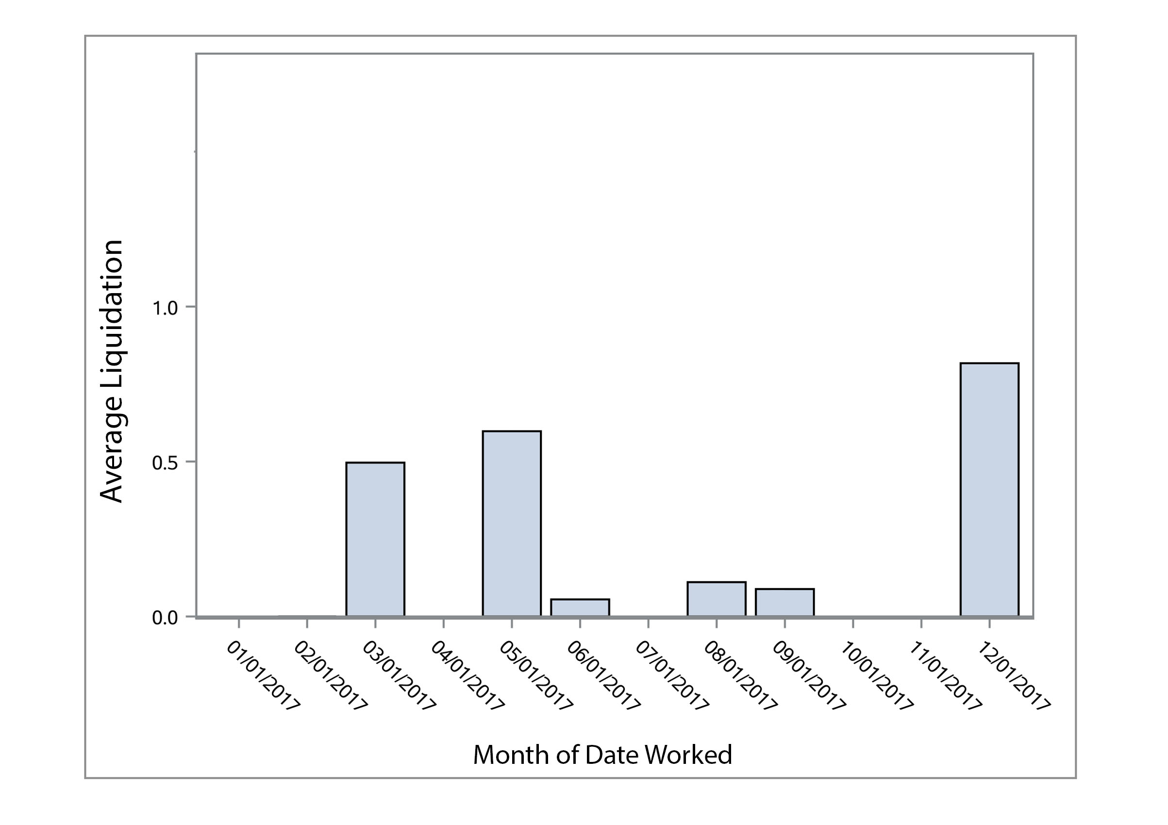
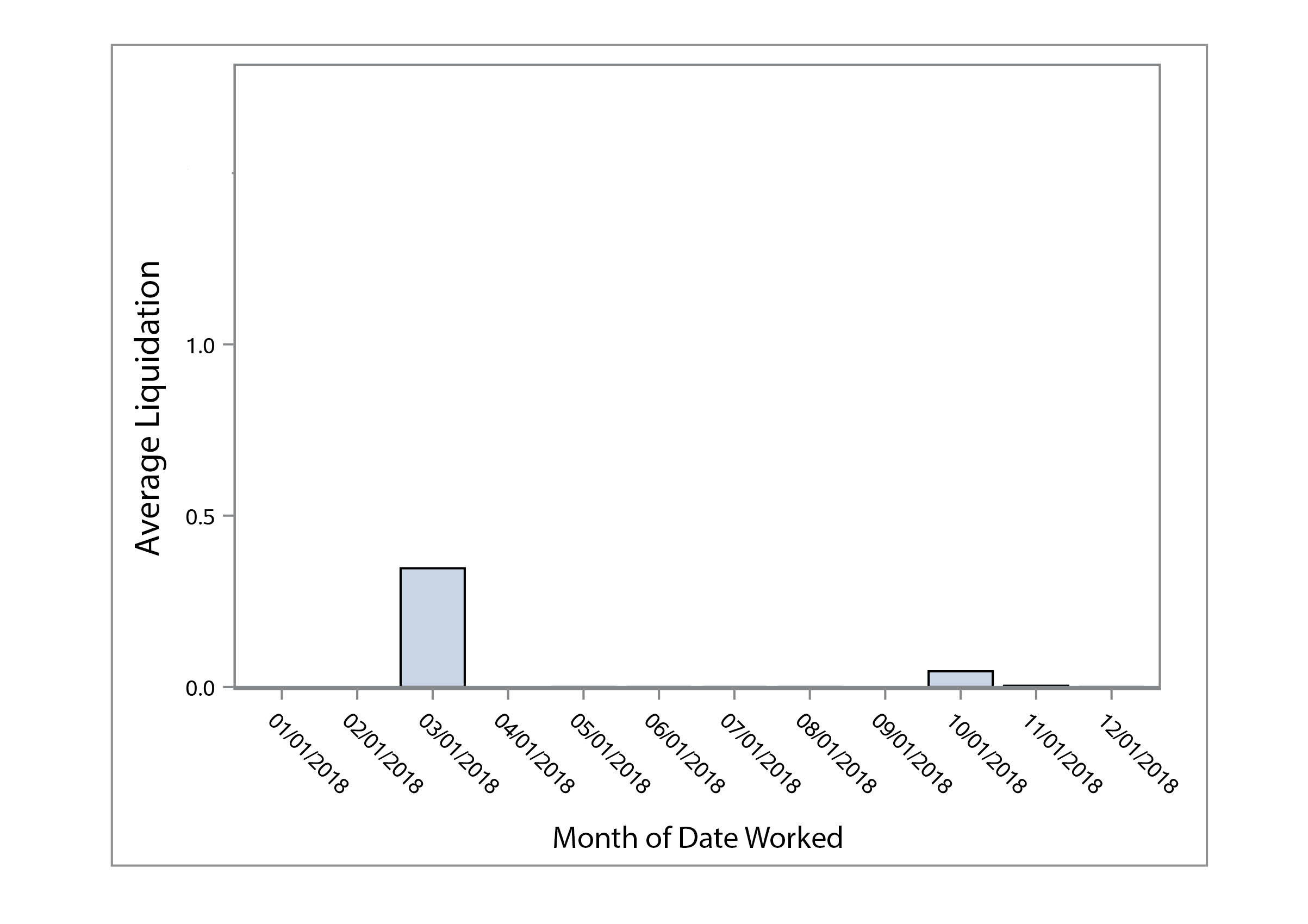
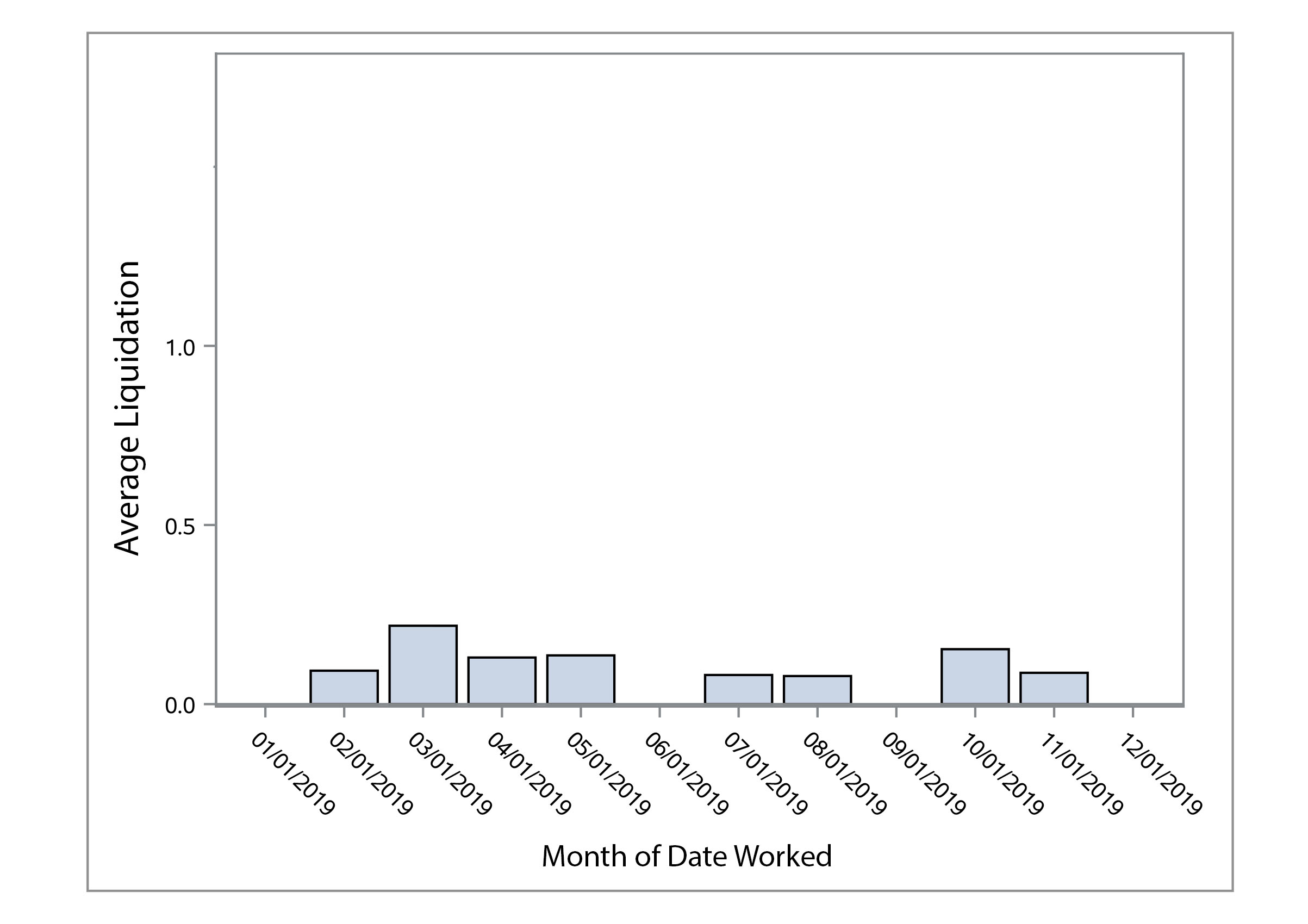
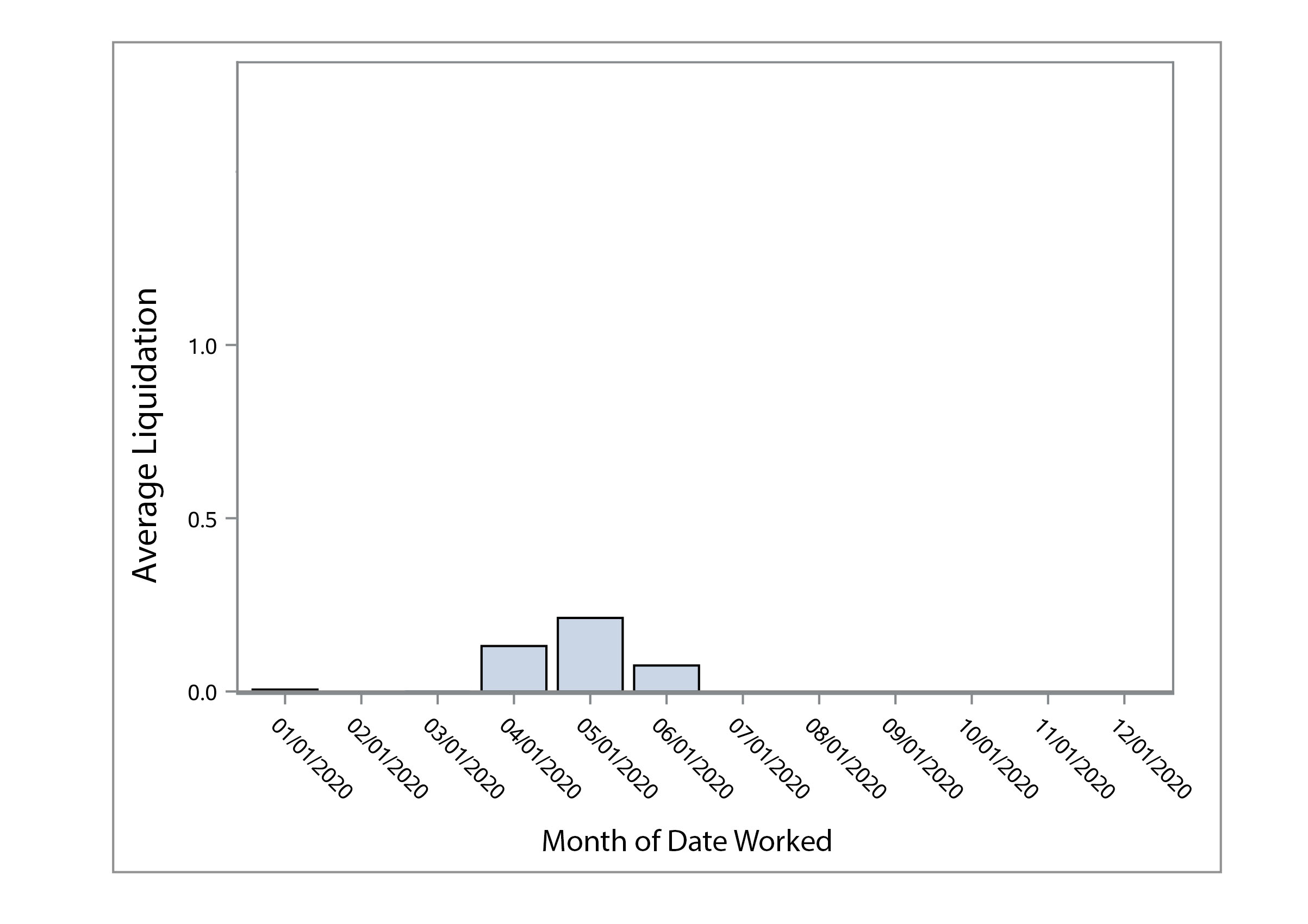
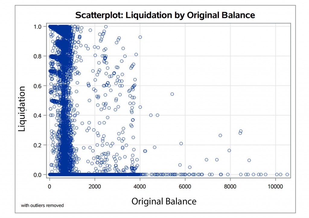
We first analyzed the data by making some visualizations to look for trends or outliers. Below you can see plots for average liquidation by month worked for the years 2017 – 2020. We thought some months would have a higher liquidation than others, but there did not seem to be a clear trend or any seasonality in the amount collected.
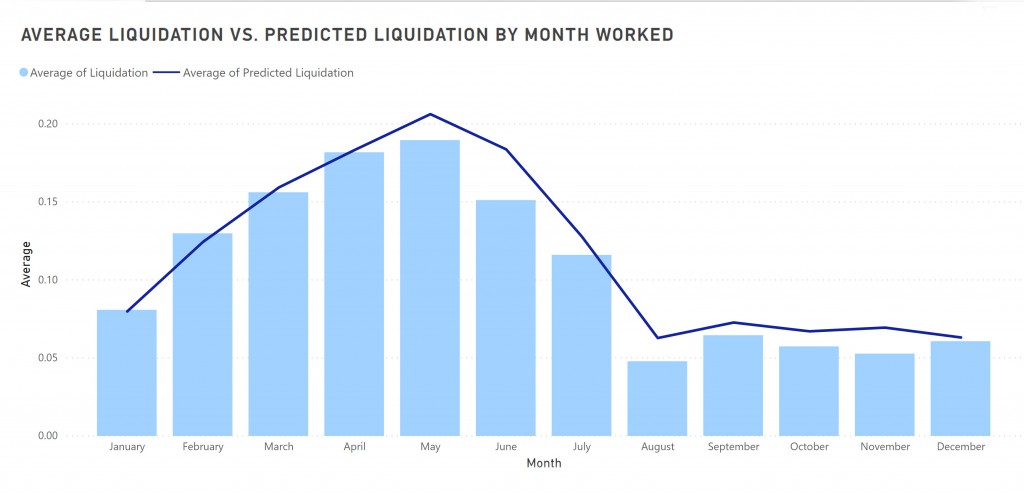
This images shows our predicted outcomes for liquidation by month worked versus the actual outcomes from the test data set. Our model predicted fairly close to the actual outcomes.
| Model Significance | Model R2 | RMSE Calculation for Prediction |
|---|---|---|
| <.0001 | .233 | .27452 |
Regression analysis results and RMSE calculation for prediction vs actual values.
This project shows my level of understanding in using SAS to run a regression analysis and work with real data.
Impact:
XYZ will be able to make better decisions when looking to purchase a new portfolio based on their ability to reach a certain % liquidity. XYZ will be able to negotiate a better price for the charged-off accounts, if they know the probability of being able to collect a certain amount.
Sample Code
Data Engineering
*This code changes input to a SAS date format that looks like 02/01/2001 instead of a random number code. This makes the sgplot code for for the date graphs easier to read;
data combine;
set combine;
format DateWorked1 mmddyy10.;
format ChargeOffDate1 mmddyy10.;
Visualizations in SAS
*Bar charts for year 2017. This takes the mean of the liquidation for the month;
proc sgplot data=WORK.COMBINE;
vbar Dateworked1 / response=Liquidation1 stat=mean;
format date MONYY.;
xaxis values=(‘1jan17’d to ’31dec17’d by month);
run;
Regression analysis and prediction outputs
*model: calibrate is the partition of 80% of the data set;
proc glm data=calibrate;
class State DateWorked1;
model Liquidation1 =OriginalBalance1 AverageHomeValue1 AverageIncome1 Difference State DateWorked1/solution;
store out=model3;
run;
proc plm source=model3;
score data=predict out=modelproject3 pred=predliq1;
run;
data temp3; set modelproject3;
error=Liquidation1-predliq1;
sqerror=error*error;
run;
proc means data=temp3;
var sqerror;
OUTPUT OUT=temp3_2 MEAN= ;
run;
data temp3_2; set temp3_2;
rename sqerror=mean_sqerror;
run;
data temp3_2; set temp3_2;
rmse3=(mean_sqerror**0.5);
run;
proc print data=temp3_2;
var rmse3;
run;

